Full parallelisation and modernisation of the BGS global magnetic field model inversion code

eCSE10-12

Key Personnel

PI/Co-I: Susan Macmillan (PI, BGS), Brian Bainbridge (Co-I, BGS), Nick Brown (Co-I and technical, EPCC), Ciarán Beggan (Co-I, BGS)

Technical: Nick Brown (EPCC)

Relevant documents

eCSE Technical Report: Full parallelisation and modernisation of the BGS global magnetic field model inversion code

Project summary

The BGS global geomagnetic model inversion code is used to produce various models of the Earth's magnetic field. It is essentially a mathematical model of the Earth's magnetic field in its average non-disturbed state. The input consists of millions of data points collected from satellite and ground observatories on or above the surface of the Earth which are used to identify the major sources of the magnetic field: the core, crust, ionosphere and magnetosphere. The magnetic field is then solved for the so-called Gauss coefficients, which describe the magnetic field as weighting factors for spherical harmonic functions of a certain degree and order (ie spatial wavelength). In addition, the Gauss coefficients have a temporal dependence requiring the solution of weights for a sixth-order B-spline function. The output is thus a set of around 10,000 coefficients describing the spatial and temporal variation of the magnetic field from the core to near-Earth orbit over a period of around 15 years. This allows a compact representation of the magnetic field.

Figure 1 - (Left) Magnetic Declination angle for 2015.0 for the Earth's main field to degree and order 13. (Right) Lithospheric magnetic field strength for degree and order 16 to 133 (in nanoTesla).

A partial parallelisation of the model had been performed, but this is based on decomposing the input data, building up a matrix on each process and then summing values from distinct processes to calculate contributions. Crucially the matrix size is the square of the number of parameters, which must be allocated on each process, and so memory limits are hit as the size of the problem increases. The scientists would now like to study much larger systems, but crucially the memory limits of the model inhibit this.

In this project we have entirely replaced the parallelisation with a new approach that decomposes on the matrix rather than the input data. We have also replaced the bespoke sequential solver of the previous code with the SLEPc and PETSc library, which not only provides numerous possible solvers out of the box but also gives parallelisation for free. The code has been modernised, entirely updated from fixed-form FORTRAN 77 to modern, free-form Fortran 90. This is important as not only does it make it far easier to understand and maintain, but it also enables other good software engineering practice such as documentation and coding standards to be applied.

The results of this work are a model whose results match very closely with the previous model but performs orders of magnitude faster. This work has the potential to produce a step change in modelling the Earth's geomagnetic environment by providing both the capability to model much larger systems and the flexibility for end users to select the most appropriate solver for their problem.

Achievement of objectives

The objectives of the work were to:

Metric One: The ability for the code to run on at least 1,000 cores with reasonable scaling/parallel efficiency. The runtime of the code on 112 cores of the BGS machine (for a specified data set/test-case) is around 11 hours. This contains a significant serial fraction and if the code was completely parallelized the runtime should be significantly reduced. Strong scaling wise, we are aiming for a baseline of max 8.5 hours runtime.

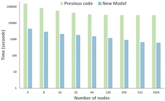
Figure 2 - Performance comparison of previous and new model with system size of 10,339 parameters and 4.3 million data points. The new model is 51 times faster at 1024 nodes than the previous model.

Figure 2 illustrates the performance and scaling of our new model against the previous model, for the standard problem size we used in the proposal. It can be seen that the runtime has very significantly decreased, even at a modest number of nodes the runtime is well within our metric limit (eg runtime of 29 minutes over 32 nodes, well within the 8.5 hours target!). Figure 2 illustrates runs out to 1024 nodes (24,576 cores), which very convincingly beats our target of running on at least 1000 cores. The runtime at this scale is 8 minutes.

Metrics Two and Three: Provide the ability to solve over 100,000 parameters (Metric Two), and solve the 100,000 parameter task in 240 hours or less (Metric Three).

This target was most challenging due to unforeseen issues with SLEPc and memory usage. As detailed in the technical report, internal memory inside a specific process used by SLEPc increases significantly as the system size is scaled. Crucially this does not parallelise, so adding more cores doesn't help at all here. Numerous SLEPc settings were tried, including setting the maximum project dimension and alternative parallel direct linear solvers such as MUMPS. However none of these reduced the memory overhead.

We adopted two ways to get around this problem. The first is simply a matter of time: ARCHER is an old machine, and the 64GB per node is a small amount of memory in comparison with that provided by more modern machines. For instance the Tier-2 machine Cirrus has 256GB per node, and we used it for some of the larger system sizes in our experiments.

This memory penalty is on a process-by-process basis, and so the other approach we adopted was to add OpenMP to add threading inside a process. This made it possible to run one process per NUMA region and hence the memory penalty is then per NUMA region rather than per core without a loss in performance (actually this can improve performance due to better use of the L3 cache!).

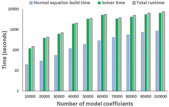
Figure 3 - Scaling the number of model coefficients over 40 nodes of ARCHER

The timing results of 100,000 model coefficients (illustrated in Figure 3) is well within the target 240 hours of the metric. It should be noted that a parameter size of 100,000 requires the matrix to hold 10 billion entries, and this is a very large number. PETSc must be compiled with 64-bit addressing enabled, and even using the 256GB of Cirrus it is not currently possible to solve the eigenvalue problem for a parameter size this large. Instead, we split the problem up into two chunks, each 50,000 parameters, and solve these individually before combining the results.

As it currently stands this is a reasonable workaround, and well within the time limit of this metric (see technical report), but for much larger systems we suggest moving to an iterative rather than direct method for the solver. Crucially the work done in this project means that it is trivial, using PETSc, to swap one out for the other at the code level, and-so the main challenge here is one from the BGS's perspective in terms of correctness and tweaks to the equations as required.

Metric Four: Along with previous performance metrics, results should be in agreement (eg within a relative 0.1%) with the results produced by the current code on ARCHER and BGS facilities.

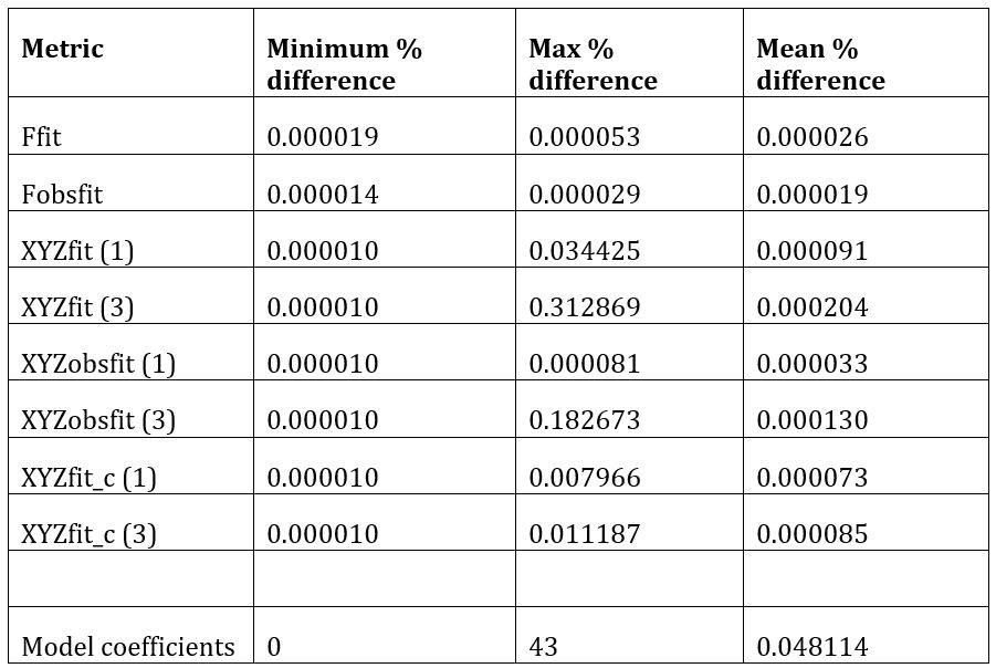
Table 1 - Percentage result difference between results generated by previous model and new model with experiment of figure 1 over 32 nodes

Table 1 illustrates a comparison between the results obtained by the BGS's existing model and our new model, based on the standard test used in the proposal. Even though the code has been entirely re-written in modern free-form Fortran and uses an entirely different solver package, it can be seen that we are well within the 0.1% difference of the metric. The vast majority of result files exhibit tiny differences, the reason for the larger number in the model coefficients are some very tiny numbers smaller than 1e-30. After discussions with the BGS it was determined that, whilst these differences might seem significant as percentages, in reality they make no significant difference to the overall results because those numbers are so tiny.

Summary of the Software

As described in the proposal, the model developed as part of this eCSE is BSD-licensed and made freely available to the community. This is currently through a private Github repository and BGS is currently going through an internal review process before we make this a public repository (this is standard practice). This will most likely move from Github to BGS hosting, which is again standard practice for these sorts of models.

There is full documentation in the repository that describes the installation, building and usage of the model as well as helper scripts (including submission scripts on ARCHER) to assist users. The makefiles are currently set up to build with the Cray, Intel and GNU compilers on ARCHER as well as Cirrus. It is trivial to add in new build targets. There are also the lecture slides and practical exercise sheet from the BGS course we ran in December 2018.

During the course of this project we have installed SLEPc as a module on ARCHER, which avoids the need for users to manually install and configure it. Additionally there are setup scripts in the repository, so the user executes source scripts/archer_env.sh which will automatically load the appropriate modules for them. Whilst the eCSE projects are focused on ARCHER, BGS has also installed and tested the model on its own internal HPC cluster and it is also ready to go on there too.

Scientific Benefits

Each year BGS generates a model of the Earth's magnetic field environment. It currently takes over 12 hours to run this model and, based on the experiments performed for this report, BGS scientists believe that this will be cut to around 15 minutes. This is a very important impact in itself because the resulting model is used as input to a variety of other models, such as those used by BGS research activities and some BGS commercial clients. The plan will be to initially run the two models together, certainly for the first time it is run. This will enable a detailed comparison of results and provide BGS with further evidence of the soundness of results from the new model.

The significantly increased capability of our new code will enable BGS to generate its yearly model using a system that is far more accurate and detailed. In the shorter term BGS will run this model for some of its more general workloads and, based on the training course run at the BGS in December 2018, it is hoped that the wider community will also adopt and use this model.